The Transit of Venus of June 8 2004
Introduction
The transit of Venus that took place on the 8th of June 2004 was a long awaited event. The previous transit had taken place on 6th December 1882, so it is a safe assumption that no one alive in 2004 had ever seen one. Perhaps for this reason it promised to be the best observed transit of all time, attracting world wide attention. It would be a far cry from the almost solitary observations of the first transit ever seen by man, made by Englishman Jeremiah Horrocks in 1639. Along with everyone else I planned to observe the transit and take photographs of the event from my home in Cheshire.
The official times for the key moments of the transit were as follows:
First contact : 06:13.5 BST
Second contact: 06:32.8 BST
Third contact : 12:06.5 BST
Fourth contact : 12:25.9 BST
The complete event was therefore expected to last about six hours, long enough in the changeable British climate to encourage the hope of observing it for at least some of the time.
Observations
My equipment consisted of a Meade LX10 200mm F10 Schmidt-Cassegrain telescope with solar filter and a Pentax K1000 SLR camera at the prime focus. The film used was Fujicolor Superia X-tra 400 negative film. The conditions were reasonably good: cloudy at first, but becoming clear as the transit progressed and then gradually succumbing to high cloud towards the end of the transit. Because of these changing conditions the start and end of the transit were unobservable, but for most of the time, the conditions were excellent.
In all I took 34 photographs at intervals throughout the transit. A sample photograph appear below. When each photograph was taken the time according to a radio controlled clock was noted and rounded to the nearest second. The effects of changing cloud cover can be seen in some of them, but in all cases Venus can be seen on the Sun’s disc. During the session the exposure was varied at intervals in response to the light levels, but the main differences in brightness in these photographs is the result of post processing. The photographs here have been scanned in from the film negative using a PrimeFilm 1800U scanner and have been cleaned up using GIMP software.
The telescope was set up in alt-azimuth mode (for daylight observation) and the equipment was moved twice during the transit to capture the full event against an interrupted skyline, it is not possible to follow the transit as a neat progressive sequence in these photographs, as the images are rotated with respect to each other. But in the analysis reported below I have attempted and effective reconstruction of the transit.
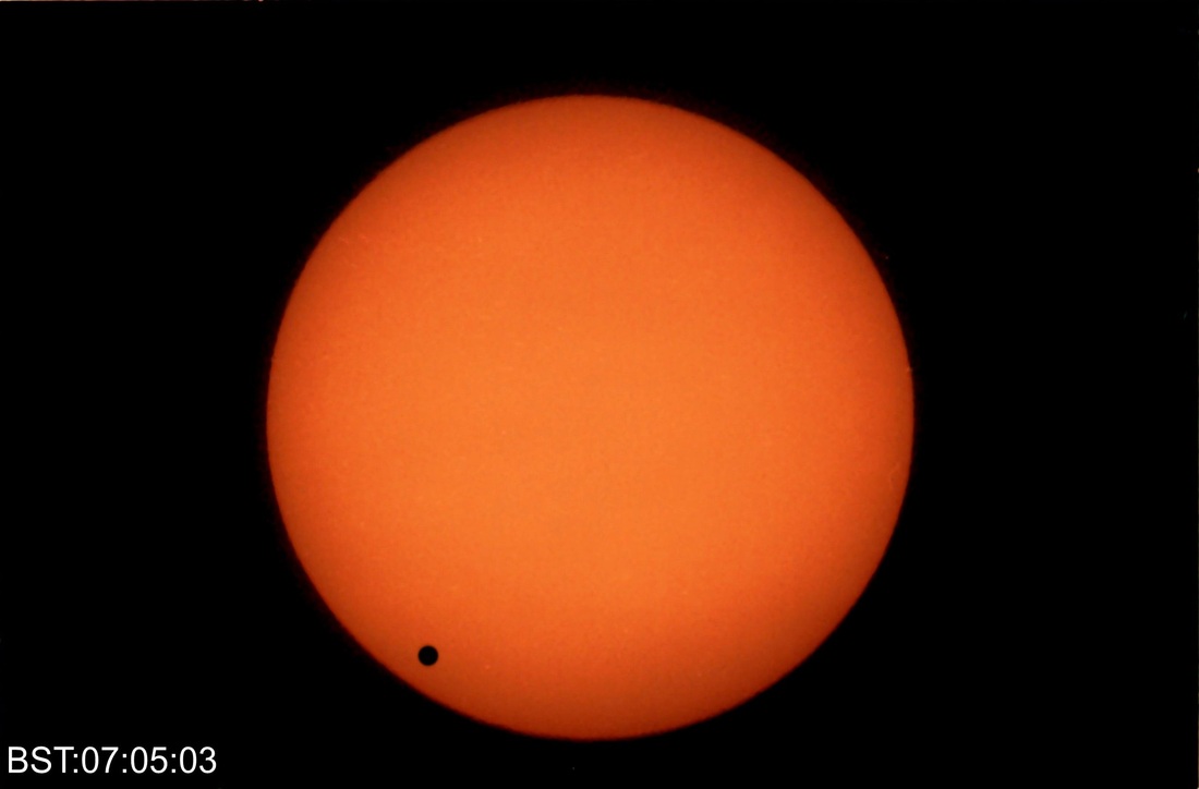
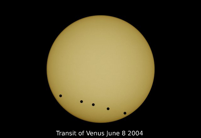
A typical Venus transit shot.
Photograph Analysis
While the photographs I took represent an interesting record of the event and would be valuable to me for that purpose alone, I was interested in trying to draw from them some scientific data. I had not been careful in positioning my tescope mount and moved it around the garden occasionally to get the best view. But I reasoned it should be possible to reconstruct the path of Venus across the face of the Sun and obtain from that estimates for the start and end times of the transit, both of which I had missed. The question was how to conduct this analysis given the fact that I did not have tools for measuring the photographs. I adopted the following approach in which I worked with positive prints of the photographs.
While the photographs I took represent an interesting record of the event and would be valuable to me for that purpose alone, I was interested in trying to draw from them some scientific data. I had not been careful in positioning my tescope mount and moved it around the garden occasionally to get the best view. But I reasoned it should be possible to reconstruct the path of Venus across the face of the Sun and obtain from that estimates for the start and end times of the transit, both of which I had missed. The question was how to conduct this analysis given the fact that I did not have tools for measuring the photographs. I adopted the following approach in which I worked with positive prints of the photographs.
- It was easy to measure the diameter of the Sun’s image on a photograph with an ordinary ruler. This was 84.3 mm which gave me a working radius for the image of 42.15 mm. This I took to be my unit of length. I also assumed the Sun’s image was a perfect circle.
- On a sheet of transparent paper I drew a circle of radius 42.15 mm with a compass and marked the centre where the compass point was located. This became a measuring template, which was used as follows;
- Laying the template over the image of the Sun in each photograph I was able to mark the position of Venus with a pencil point and so measure the distance between this point and the centre of the disc with a ruler. This gave the set of results presented in Table 1, where columns labelled `y’ record the measured distances of Venus from the Sun’s centre on each photograph. The corresponding times are also reproduced.
- I assumed that the path across the sun was a straight line. Likewise I assumed that the speed of Venus during the Transit was constant. These assumptions seemed reasonable given that this represents only about 6 hours’ of the motion of Venus from an orbital period of 224.7 days (5393 hours). Any departure from linearity on the observation timescale should be negligible. A further assumption, though not one I actually needed to use, was that the path of Venus lay in the ecliptic.
- A least squares analysis was performed on the data in Table 1 to provide the best fit of the data as a quadratic function of time (see theory below). The resulting fit represents the required calculated trajectory.
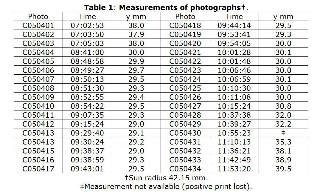
A comment on Table 1 is worth making. It is apparent that the observations are clustered in time, as 3 distinct clusters occur from 7:02 to 7:05; 8:41 to 10:15; and from 10:37 to 11:53. Within each cluster the variation in the measured distance Y is quite small, and the method of measurement does not seem to be able to distinguish very well between adjacent points. However across all three clusters there are significant differences and I was hopeful that the least squares procedure would provide a reasonable fit overall.
Theory
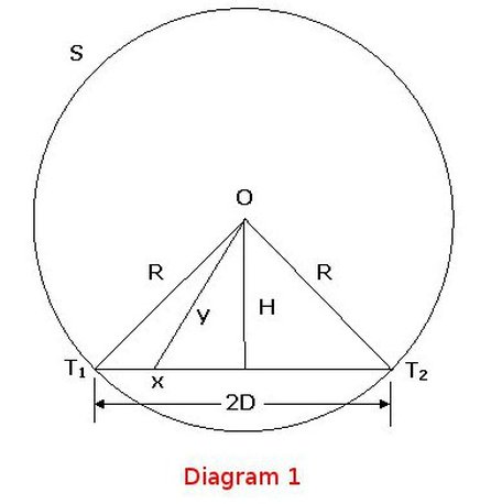
In Diagram 1, S represents the disc of the Sun in a photograph, with centre at O. Line T1 – T2 represents the track of Venus, which is an assumed straight line of length 2D. Lines labelled R are radii of the Sun’s disc and H is a perpendicular dropped from O to the line T1 – T2, which is thus bisected. The line y represents the distance of Venus from O (as given in Table 1) and x represents the distance travelled by Venus along the line T1 – T2. Now we have by Pythagoras’ theorem:
H^2 = R^2 - D^2 = y^2 - (D - x)^2. (1)
So
R^2 - D^2 = y^2 - D^2 + 2Dx – x^2. (2)
Hence
x^2 – 2Dx + R^2 = y^2. (3)
At this point we can simplify things a little if we assume that all our distances are measured using the radius of the Sun’s image as the unit of length, which means that R=1 and y is the equivalent fraction of the Sun’s image radius (i.e. we divide our measured value of y in mm by the radius of the Sun’s image in mm, so y < 1 always). This also has the advantage of making our analysis independent of the size of photograph we are using to obtain our results. Now we have:
x^2 – 2Dx + 1 = y^2. (4)
Also we assume that:
x = vt + g, (5)
where v is the constant velocity of Venus across the Sun’s disc, t is the time and g is a constant. This is the linear motion assumption. We can also write the square of this formula:
x^2 = (vt)^2 + 2vtg + g^2. (6)
Combining the above 3 equations we obtain:
(vt)^2 + 2vt(g – D) + g^2 - 2Dg + 1 = y^2, (7)
which we may write as
At^2 + Bt + C = y^2. (8)
This is a quadratic equation in time (t) describing the variation in the measured variable y as Venus moves along the assumed linear path across the Sun’s disc. We should also note that:
A = v^2
B = 2v(g – D) (9)
C = g^2 – 2Dg +1
The intention is to fit equation (8) to the data in Table 1 using Gauss’ method of least squares. This provides the values of the constants A, B and C which best fit the data. From these constants we can use the relations (9) to obtain the speed v, the distance D and the position g that define the path of Venus across the Sun’s disc. Thus (9) can be rearranged as follows:
v = √A
D = (B^2 – 4 A [C-1])^(1/2) /2√A (10)
g = B/2√A + D
I have performed these calculations using a quadratic least squares routine I wrote myself. The results are as follows:
A = 0.06495871, B = -0.3046565, C = 0.8320770
From which I obtained:
v = 0.25487, D = 0.72466, g = 0.12700
(I should mention here that I subtracted 7 hours from the timings reported in Table 1, so that all time measurements were defined with respect to a time origin at 7:00am. This is largely a matter of convenience, but it does also help a little with numerical accuracy. Getting the true times for events is simply a matter of adding back the 7 hours later.)
How well these parameters fit the data supplied can be seen from Table 2.
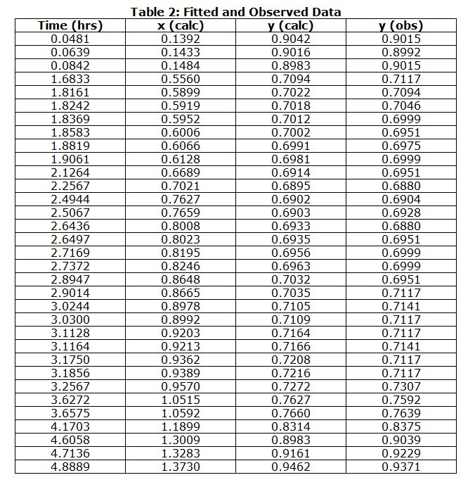
The first two columns of Table 2 give the times (column 1) and corresponding positions (column 2) of Venus along the straight line representing the transit path. The transit path, is a cord of the circle representing the Sun’s disc, and has a length of 2D, or 1.44932 times the radius of the Sun (on whatever scale you wish to draw it). The times are in decimal hours, to which 7 hours must be added to get the clock time (BST). The distance x is zero when the centre of Venus lies on the edge of the Sun’s disc at the start of the transit. At the opposite end x has the value 1.44932, when the centre of Venus crosses the Sun’s edge to signal the end of the transit.
Table 2 also shows both the observed value of the variable y (as a fraction of the Sun image disc radius) and the calculated value based on the best fit parameters above. The RMS error averaged over all points is 0.00487, or about half of one percent.
The start and end times of the transit may be calculated from equation (5) (recall that 7 hours must be added to the result).
When x=0, then the time in hours is:
t_start = 7 - g/v = 7 - .127/.25487= 7 - .498293 = 6:30:06.
This should be compared with the estimated start time (obtained as the mean of the first and second contacts), which is 6:22:57.
When x=2D, meaning the end of the transit, (i.e. x= 1.44932), then
t_finish = 7 + (2D - g)/v = 7 + (1.44932 - .127)/.25487 = 12:11:18.
This should be compared with the estimated finish time (obtained as the average of the third and fourth contacts), which is 12:16:12.
The duration of the transit is the difference between the finish and start times:
t_duration = 5:41:11.
The comparable time from official calculations is 5:54:15. Thus my calculation of this is in error by 3.7%, compared with published data.
On an historical note, the calculation of t_duration, was suggested by Halley as a possible means for calculating the parallax of Venus and from that, the Sun. The idea was that t_duration should be calculated for several observation stations scattered across the world. The amount by which these differed from each other, for known positions on Earth, would indicate the parallax of Venus. Other methods included the measurement of times of the second or third contacts, from different locations, which would also indicate the parallax. Halley’s method is a little more reliable, since it depended less on the precise determination of a single event. By such methods the size of the solar system was first calculated with reasonable accuracy.
To finish off I present below a composite of several images of the transit, highly reworked with image processing software, and realigned using information obtained by the above analysis. It makes a nice record of the event.
Reconstruction of the transit of Venus using multiple images.
Conclusion
A measurement of the distance of the image of Venus from the centre of the image of the Sun, was fitted using least squares to a quadratic function of time, assuming a uniform, linear progression of the disc of Venus across the face of the Sun. By these fairly rough methods it has been possible to get a reasonable estimate of the start, duration and end times of the transit of Venus.
